Bose–Einstein Condensation without an Initial Low-Energy Concentration Assumption

Introduction

Model and condensation problem

Bose–Einstein condensation (BEC) is a quantum collective phenomenon: at sufficiently low temperature, a macroscopic fraction of bosonic particles may accumulate in the lowest-energy state. The phenomenon originates from Bose’s quantum statistics for indistinguishable particles and Einstein’s extension of this statistics to an ideal gas of material particles, which led to the prediction of the condensation transition [Bos24, Ein24, Ein25]. A mesoscopic kinetic model for Bose–Einstein particles is the spatially homogeneous quantum Boltzmann equation \[\partial_t f(v,t) = \int_{\mathbb R^3}\int_{\mathbb S^2} B(v-v_*,\omega) \bigl[ f'f_*'(1+f)(1+f_*) - ff_*(1+f')(1+f_*') \bigr] \,d\omega\,dv_*,\tag{1.1}\] where \(f=f(v,t)\geq0\) is the particle number density at time \(t\) and velocity \(v\), with \[f_*=f(v_*,t),\qquad f'=f(v',t),\qquad f_*'=f(v_*',t),\] and the post-collisional velocities are \[v'=v-\bigl((v-v_*)\cdot\omega\bigr)\omega, \qquad v_*'=v_*+\bigl((v-v_*)\cdot\omega\bigr)\omega, \qquad \omega\in\mathbb S^2.\] The quantum Boltzmann equation for Bose particles goes back to Nordheim [Nor28] and Uehling–Uhlenbeck [UU33]. Its derivation from microscopic quantum dynamics and its mathematical theory have been studied in a variety of settings; see, among others, [BCEP05, Lu04, Lu05, BE16, LL19]. A characteristic feature of (1.1), different from the classical Boltzmann equation, is the appearance of the Bose-enhancement factors \(1+f\). According to Bose statistics, the presence of particles in a given one-particle state increases the probability that further particles enter the same state. Thus, in a binary collision, transitions into the states \(v\) and \(v_*\) are enhanced by the factors \((1+f)(1+f_*)\), while transitions into \(v'\) and \(v_*'\) are enhanced by \((1+f')(1+f_*')\). This statistical amplification of already occupied states is the basic quantum mechanism through which the collision dynamics can drive particles toward highly occupied low-energy states. For isotropic solutions, we can use the kinetic-energy variable \(x={|v|^2}/{2}.\) In the corresponding measure-valued formulation \(F_t(dx)\), Bose–Einstein condensation is represented by the appearance of a nonzero atom at the zero-energy state \(x=0\). Below the critical temperature \(\overline T_c\), the Bose–Einstein equilibrium contains such a zero-energy atom, and this leads to a fundamental question in dynamics: given an initial state whose mass and energy correspond to a temperature below the critical temperature, can the collision dynamics create a condensate at \(x=0\), and can this happen in finite time? For the hard-sphere Nordheim equation, finite-time condensation was established by Lu under assumptions on the initial concentration near zero energy [Lu13, Lu14]. Escobedo and Velázquez then established condensation results for general measure-valued initial data under the only assumption \(\overline T/\overline T_c<1\) [EV14, EV15]. At the same time, the interaction potential has a significant impact on both the occurrence of Bose–Einstein condensation and its long-time convergence. To make the role of the particle interaction more explicit, we now specify the collision kernel. In the weak-coupling regime, microscopic derivations of the quantum Boltzmann equation lead, after a normalization of physical constants, to a collision kernel of the form [BCEP05, ESY04] \[B(v-v_*,\omega) = \frac{|(v-v_*)\cdot\omega|}{(4\pi)^2} \Phi\bigl(|v-v'|,|v-v_*'|\bigr),\tag{1.2}\] where, for a real radially symmetric two-body interaction potential \(\phi=\phi(|x|)\), \[\Phi(r,\rho) = \bigl(\widehat\phi(r)+\widehat\phi(\rho)\bigr)^2, \qquad r,\rho\geq0.\tag{1.3}\] Here \(\widehat\phi\) denotes the radial Fourier transform of \(\phi\). The two terms in (1.3) correspond to the direct and exchange scattering amplitudes for identical bosons, and thus the low-momentum behavior of \(\widehat\phi\) directly determines the strength of collisions near zero energy. The hard-sphere model is obtained from the constant choice \(\widehat\phi\equiv1/2\), for which \(\Phi\equiv1\) and \[B(v-v_*,\omega) = \frac{1}{(4\pi)^2}|(v-v_*)\cdot\omega|.\] Cai and Lu [CL19] studied a class of such kernels for which \(\widehat\phi\) is continuous and nondecreasing and, for some \(b_0>0\) and \(0\leq\eta<1/4\), satisfies \[b_0\frac{r^\eta}{1+r^\eta} \leq \widehat\phi(r)\leq\frac12, \qquad r\geq0.\] For \(0\leq\eta<1/4\), they proved strong convergence to the Bose–Einstein equilibrium under the standard low-temperature condition \(\overline T/\overline T_c<1\), without imposing local assumptions on the initial distribution near zero energy. Their recent work [CL26] isolates the properties of the scattering cross section and treats a broader class of kernels in which the scattering factor \(\Phi\) need not be explicitly generated by an interaction potential. In particular, they quantify the possible degeneracy of \(\Phi\) at low momentum transfer through an exponent \(\eta\): for \(0\leq\eta<1\), their condensation theory assumes the lower bound \[\Phi(r,\rho)\geq b_0\min\{1,(r^2+\rho^2)^\eta\},\] with the symmetry and monotonicity properties of \(\Phi\). Thus larger values of \(\eta\) allow a stronger weakening of the collision interaction as \((r,\rho)\to(0,0)\). Under this assumption, they obtained convergence to Bose–Einstein condensation and strong convergence for \(0\leq\eta<1\) provided the initial data satisfy an additional quantitative low-energy concentration condition. Indeed, with \(0<\alpha<1-\eta,\beta=(1-\eta-\alpha)/2\), and \(p=3/2+\alpha\), they suppose that the initial value \(F_0(dx)\) in energy variable satisfies \[\begin{aligned}\inf_{0<\delta\leq 2E/N}\dfrac{F_0([0,\delta])}{\delta^\alpha} &\geq \dfrac{2^\alpha 18}{b_0}\left(\dfrac{4\sqrt2}{3-p}\right)^2\left(\dfrac p \beta\right)^{2p}\left(\dfrac {4E}N\right)^{1/2+2\beta}\max\left\{\dfrac{4E}{N},1\right\}^\eta,\\ N &=\int_{[0,\infty)} dF_0(x),\qquad E=\int_{[0,\infty)}x\,dF_0(x).\end{aligned}\tag{1.4}\] This in particular forces the ultra-low-temperature bound \[\dfrac{\overline T}{\overline T_c}<\frac{1}{600}b_0^{2/3}(1-\eta)^2.\tag{1.5}\] In the opposite direction, under their corresponding upper-degeneracy assumption with \(\eta\geq1\), they showed that an initially absent zero-energy atom cannot be dynamically created. Motivated by this threshold behavior, and following their formulation in the range \(0\leq\eta<1\), we impose the following assumption.

Our main result removes the additional initial low-energy concentration condition (1.4) for the full range \(0\leq\eta<1\). For \(0\leq\eta<1/4\), this conclusion was already obtained in [CL19]; thus the new range is \(1/4\leq\eta<1\). Consequently, the admissible temperature range is extended from the ultra-low regime (1.5) to the full subcritical range \(\overline T/\overline T_c<1\). More precisely, once the mass and energy correspond to a Bose–Einstein equilibrium below the critical temperature, semi-strong relaxation to that equilibrium, proved in [CL26], forces a nonzero zero-energy atom to be present after a finite time. The condensate mass then converges to its equilibrium value, and the full solution converges strongly to the Bose–Einstein equilibrium.

Basic concepts and notation

We work throughout the paper with the isotropic formulation in the energy variable \(x={|v|^2}/{2}\in[0,\infty)\) in 3D, and denote by \(F_t(dx)\) the corresponding nonnegative energy measure at time \(t\). In this formulation, Bose–Einstein condensation is represented by the appearance of an atom at zero energy. Denote the condensate mass by \(N_c(t):=F_t(\{0\}),\) and write \[F_t=N_c(t)\delta_0+F_t^{\circ}, \qquad F_t^{\circ}(\{0\})=0,\tag{1.7}\] where \(F_t^{\circ}\) denotes the non-condensed part of the measure. Whenever the non-condensed part is absolutely continuous with respect to \(\sqrt{x}\,dx\), we write \[dF_t(x) = g_t(x)\sqrt{x}\,dx+N_c(t)\delta_0(dx).\tag{1.8}\] In particular, if the isotropic velocity distribution has the form \(f(v,t)=g_t({|v|^2}/{2})\), its absolutely continuous energy measure is \(g_t(x)\sqrt{x}\,dx\) after dividing out the radial factor \(4\pi\sqrt2\). For a nonnegative Borel measure \(F\) on \([0,\infty)\) with finite mass and finite first moment, we denote its particle number and energy by \[N(F):=\int_{[0,\infty)}dF(x), \qquad E(F):=\int_{[0,\infty)}x\,dF(x).\tag{1.9}\] For a conservative solution \((F_t)_{t\geq0}\), both quantities are independent of time, and we simply write \[N:=N(F_t), \qquad E:=E(F_t).\] We consider the space of measures \[\mathcal B_1^+([0,\infty)) := \left\{ F:\ F\ \text{is a nonnegative Borel measure on }[0,\infty), \quad \int_{[0,\infty)}(1+x)\,dF(x)<\infty \right\}.\tag{1.10}\] Thus \(F\in\mathcal B_1^+([0,\infty))\) precisely when both \(N(F)\) and \(E(F)\) are finite. For particle number \(N>0\) and energy \(E>0\), we denote by \(\overline T\) the temperature determined by particle number and energy, and by \(\overline T_c\) the corresponding critical temperature for Bose–Einstein condensation. In the normalization adopted here and in [CL26], \[\frac{\overline T}{\overline T_c} = \frac{(2\pi)^{1/3}[\zeta(3/2)]^{5/3}} {3\zeta(5/2)} \frac{E}{N^{5/3}},\tag{1.11}\] where \(\displaystyle \zeta(s)=\sum_{n\ge 1}n^{-s}\) is the Riemann zeta function. Accordingly, \({\overline T}/{\overline T_c}<1\) is the subcritical-temperature regime for Bose–Einstein condensation. Since \(N\) and \(E\) are conserved, the ratio \(\overline T/\overline T_c\) is fixed along the evolution. We denote by \(F_{\rm be}\) the Bose–Einstein equilibrium having the same particle number \(N\) and energy \(E\) as the solution. Its measure representation is \[dF_{\rm be}(x) = g_{\rm be}(x)\sqrt{x}\,dx + N_c\,\delta_0(dx), \qquad g_{\rm be}(x) = \frac{1}{A e^{x/\kappa}-1},\tag{1.12}\] where \(A\geq1\) and \(\kappa>0\) are determined by \(N\) and \(E\) [Lu04, CL26]. When \(\overline T/\overline T_c\leq1\), one has \(A=1\), and the equilibrium condensate mass is \[N_c:=F_{\rm be}(\{0\}) = \left( 1- \left(\frac{\overline T}{\overline T_c}\right)^{3/5} \right)_+N, \qquad a_+:=\max\{a,0\}.\tag{1.13}\] In particular, \[N_c>0 \iff {\overline T}/{\overline T_c}<1.\tag{1.14}\] For a signed Borel measure \(\mu\) on \([0,\infty)\), we define \[\|\mu\|_1^\circ := \int_{[0,\infty)}x\,d|\mu|(x), \qquad \|\mu\|_1 := \int_{[0,\infty)}(1+x)\,d|\mu|(x).\tag{1.15}\] The quantity \(\|\cdot\|_1^\circ\) is a seminorm without information for mass concentration at \(x=0\). We refer to convergence with respect to \(\|\cdot\|_1^\circ\) as semi-strong convergence, and to convergence with respect to \(\|\cdot\|_1\) as strong convergence. We use the following conventions throughout the paper. For nonnegative quantities \(X\) and \(Y\), the notation \(X\lesssim_{\mathbf p}Y\) means that \(X\leq C_{\mathbf p}Y\) for a constant \(C_{\mathbf p}>0\) depending only on the parameters listed in \(\mathbf p\), while \(X\asymp_{\mathbf p}Y\) means that both \(X\lesssim_{\mathbf p}Y\) and \(Y\lesssim_{\mathbf p}X\) hold. When the subscript is omitted, the comparison constant is independent of all quantities varying in the estimate. Similarly, \(O_{\mathbf p}(1)\) denotes a quantity bounded in absolute value by a constant depending on \(\mathbf p\). Such constants may change from line to line. We write \(a\wedge b=\min\{a,b\}\), \(\mathbf 1_A\) for the indicator of a set \(A\), \(\operatorname{supp}\varphi\) for the support of \(\varphi\), and \[\operatorname{Lip}(\varphi) =\sup_{x\ne y}\frac{|\varphi(x)-\varphi(y)|}{|x-y|}\] for its Lipschitz seminorm. Finally, \(\delta_0\) denotes the Dirac measure at zero, \(|\mu|\) the total-variation measure of a signed measure \(\mu\), and \(\mathrm i=\sqrt{-1}\).

Main results

After introducing the notations, we can now state our main results rigorously. Our first theorem shows that once a conservative isotropic measure solution relaxes semi-strongly toward a Bose–Einstein equilibrium while \(\overline T/\overline T_c<1\), a zero-energy atom is present after some finite time. Moreover, the condensate mass converges to its equilibrium value, and the semi-strong convergence is upgraded to strong convergence.

We next combine Theorem 1.2 with the existence and semi-strong relaxation theory of Cai and Lu [CL26]. This gives a finite-time condensation result for arbitrary admissible initial data in the entire range \(0\leq\eta<1\).

Strategy of the proof

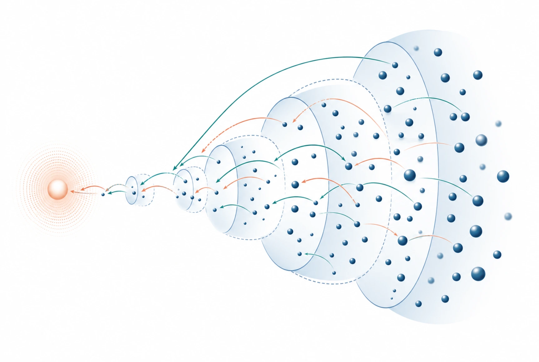
Fix \(h\in(0,N_c)\). For \(\varepsilon>0\), set \[\varphi_\varepsilon(x) =\left(1-\frac{x}{\varepsilon}\right)_+^2, \qquad N_{0,2}(F,\varepsilon) =\int_{[0,\infty)}\varphi_\varepsilon(x)\,dF(x),\] as in (2.15). For every fixed \(\varepsilon>0\), we show that semi-strong relaxation to \(F_{\rm be}\), provided by [CL26], implies \(N_{0,2}(F_t,\varepsilon)\geq h\) for all sufficiently large \(t\); see Theorem 6.2. We first choose a sufficiently small dyadic scale \(\varepsilon_j\) and then a time \(t_0\) such that \(N_{0,2}(F_{t_0},\varepsilon_j)\geq h\). Writing \(c_0=\sqrt{NE}\), the persistence estimate (3.7) then gives \[N_{0,2}(F_t,\varepsilon_j) \geq e^{-c_0(t-t_0)}h, \qquad t\geq t_0.\] To examine the collision dynamics below \(\varepsilon_j\), introduce the dyadic energy scales and shells \[\varepsilon_k=2^{-k-4}, \qquad S_k=(\varepsilon_{k+1},\varepsilon_k], \qquad A_k(t)=F_t(S_k).\] Thus \(A_k(t)\) is the mass in the \(k\)-th shell. We also choose \[m_k=4\left(1+\log\frac1{\varepsilon_k}\right), \qquad s_k=\frac{\varepsilon_k}{4m_k},\] so that \(L_k=m_ks_k=\varepsilon_{k+2}\), and use the convex cutoff \(\psi_{s,m}(x)=(e^{-x/s}-e^{-m})_+^2,\) whose properties are recorded in Theorem 4.1. At scale \(k\), set \[U_k(t) =\int_{[0,\infty)}\psi_{s_k,m_k}(x)\,dF_t(x)\] as in (5.2). The function \(\psi_{s_k,m_k}\) is supported in \([0,\varepsilon_{k+2}]\), strictly below \(S_k\), and satisfies \(\psi_{s_k,m_k}\leq\varphi_{\varepsilon_{k+2}}\) by Theorem 4.1. Hence \(U_k(t)\) is a weighted moment of the mass below the \(k\)-th shell and \(U_k(t)\leq N_{0,2}(F_t,\varepsilon_{k+2}).\) For all sufficiently large \(k\), the one-scale estimate (5.7) gives \[U_k'(t)+c_0U_k(t) \geq \gamma_kA_k(t)^2 \left(U_k(t)+\frac{Q_k}{2}\right).\] Here \(\gamma_k>0\) and \(Q_k>0\) are the constants defined in (5.3), independent of time. The term \(\gamma_kA_k(t)^2Q_k/2\), obtained from the quadratic collision form in (4.4), is positive whenever \(A_k(t)>0\), including when \(U_k(t)=0\). The term proportional to \(U_k(t)\), obtained from the cubic collision form after controlling the error as in (4.8) and (5.6), describes the Bose-enhanced transfer of particles from \(S_k\) toward lower energy scales. We next remove the linear term \(c_0U_k\). Multiplying by the integrating factor and using \(t\geq t_0\), we obtain \[\frac{d}{dt} \left(e^{c_0(t-t_0)}U_k(t)\right) \geq \gamma_kA_k(t)^2 \left( e^{c_0(t-t_0)}U_k(t)+\frac{Q_k}{2} \right).\] Consequently, \[Z_k(t) = \log\left( 1+\frac{2e^{c_0(t-t_0)}U_k(t)}{Q_k} \right)\] satisfies \(Z_k'(t)\geq\gamma_kA_k(t)^2\) by Theorem 5.3; see also (5.9) and (5.10). For fixed \(h\), let \[\Lambda_k(h) =\log\left(1+\frac{2h}{Q_k}\right),\] as in (5.11). We say that scale \(k\) is \(h\)-complete at time \(t\) if \(Z_k(t)\geq\Lambda_k(h)\), which is equivalent to \(e^{c_0(t-t_0)}U_k(t)\geq h\); see Theorem 5.4 and (5.12). Since \(\psi_{s_k,m_k}\leq\varphi_{\varepsilon_{k+2}}\), an \(h\)-complete scale satisfies \[N_{0,2}(F_t,\varepsilon_{k+2}) \geq U_k(t) \geq e^{-c_0(t-t_0)}h.\] Thus the estimate associated with \(S_k\) gives the above lower bound for \(N_{0,2}(F_t,\varepsilon_{k+2})\). In this sense, the required transfer from \(S_k\) toward lower energies has been completed. Hence, we use \(\min\left\{1,{Z_k(t)}/{\Lambda_k(h)}\right\}\) as the completion level at scale \(k\): it is strictly less than one before the target is reached and equals one after the scale becomes \(h\)-complete. To treat all sufficiently small scales \(k\geq j\) simultaneously, we introduce \[\omega_k(h) =\left(\frac{\Lambda_k(h)}{\gamma_k}\right)^{1/2}, \qquad \Theta_j(h) =\sum_{k\geq j}\omega_k(h),\] as in (5.16), and define \[\mathcal P(t) = \sum_{k\geq j}\omega_k(h) \min\left\{ 1,\frac{Z_k(t)}{\Lambda_k(h)} \right\}\] as in (5.19), to record the completion levels of all scales \(k\geq j\). Hence \(0\leq\mathcal P(t)\leq\Theta_j(h).\) At every scale that is still \(h\)-incomplete, \(Z_k(t)<\Lambda_k(h)\), and \[\frac{d}{dt} \left( \omega_k(h)\frac{Z_k(t)}{\Lambda_k(h)} \right) \geq \frac{A_k(t)^2}{\omega_k(h)}.\] Summing over all \(h\)-incomplete scales gives \[\mathcal P'(t) \geq \sum_{\substack{k\geq j\\ Z_k(t)<\Lambda_k(h)}} \frac{A_k(t)^2}{\omega_k(h)}\] for almost every \(t\) by Theorem 5.6; see (5.21). Since \(\omega_k(h) \asymp_{h,\eta} b_0^{-1/2}(1+k)\varepsilon_k^{(1-\eta)/2}\) and \(\eta<1\), \[\Theta_j(h)<\infty, \qquad \Theta_j(h)\to 0 \quad\text{as }j\to\infty.\] We now suppose \(F_t(\{0\}) < (1-\delta)e^{-c_0(t-t_0)}h\) for some \(\delta\in(0,1/2)\) throughout a short interval after \(t_0\); cf. (6.4). Then there can be only finitely many \(h\)-complete scales at any fixed time in this interval. If no scale \(k\geq j\) is \(h\)-complete, set \(\nu(t)=j\). Otherwise, let \[\nu(t) = 2+\max\{k\geq j:Z_k(t)\geq\Lambda_k(h)\},\] as in (6.5). Persistence and \(h\)-completion then give \[N_{0,2}(F_t,\varepsilon_{\nu(t)}) \geq e^{-c_0(t-t_0)}h;\] see (6.6). Hence \[\begin{aligned} \sum_{k\geq\nu(t)}A_k(t) =F_t((0,\varepsilon_{\nu(t)}])\geq N_{0,2}(F_t,\varepsilon_{\nu(t)})-F_t(\{0\})\geq \delta e^{-c_0(t-t_0)}h. \end{aligned}\] Thus a definite amount of positive-energy mass lies in \(h\)-incomplete shells. On such an interval of length at most one, Cauchy–Schwarz and the lower bound for \(\mathcal P'\) yield \[\begin{aligned} \mathcal P'(t)\geq \sum_{k\geq\nu(t)} \frac{A_k(t)^2}{\omega_k(h)}\geq \frac{\left(\sum_{k\geq\nu(t)}A_k(t)\right)^2} {\sum_{k\geq\nu(t)}\omega_k(h)}\geq \frac{\delta^2e^{-2c_0}h^2}{\Theta_j(h)}. \end{aligned}\] Set \(\tau_j(h,\delta) = 2e^{2c_0}\delta^{-2}h^{-2}\Theta_j(h)^2\) as in (6.1). For sufficiently large \(j\), one has \(\tau_j(h,\delta)\leq1\). If \(F_t(\{0\}) < (1-\delta)e^{-c_0(t-t_0)}h\) held throughout \([t_0,t_0+\tau_j(h,\delta)]\), integration would give \[\mathcal P(t_0+\tau_j(h,\delta))-\mathcal P(t_0) \geq2\Theta_j(h).\] This contradicts \(0\leq\mathcal P(t)\leq\Theta_j(h)\). Hence a positive atom must appear during this finite interval, and the persistence estimate (3.8) keeps it positive afterward; see Theorem 6.1, particularly (6.2). Once the condensate has formed, a sliding-time application of the same argument yields \(F_t(\{0\})\to N_c\), and consequently \(\left\|F_t-F_{\rm be}\right\|_1\to0\); see (6.16)–(6.17), (6.18), and Theorem 2.7.

Organization of the paper

The rest of the paper is organized as follows. Section 2 gives the isotropic weak formulation in the energy variable and states the results from [CL26] used in the proof. Section 3 proves lower bounds for the collision kernel and for the quadratic and cubic collision forms. Section 4 applies these bounds at one fixed energy scale. Section 5 introduces \(Z_k\) at each dyadic scale and combines the resulting estimates in the weighted sum \(\mathcal P\). Finally, section 6 proves finite-time formation of a zero-energy atom, convergence of its mass, and strong convergence to equilibrium.